[SIGIR 2024] Going Beyond Popularity and Positivity Bias: Correcting for Multifactorial Bias in Recommender Systems
- References
- Paper: Paper Title
- Official Code: GitHub Repository
- Conference: SIGIR 2024
1 Overview & Problem (Motivation)
1.1 Selection Bias
우리는 실제 모집단(population)의 distribution을 알 수 없기 때문에, 표본(sample)을 추출하여 사용한다.
이 때 표본이 모집단의 distribution을 제대로 반영하지 못하는 경우, Sample에 Selection Bias가 존재한다고 할 수 있다. [Ovaisi et al. definition]
- Sampling Bias라고 일컬어도 좋을 것 같은데, “Sampling” 주체가 Algorithm이니 Selection Bias라고 하는 것 같다.
이러한 Selection Bias는 user가 특정 item과 interaction을 많이 하는 self-selection bias와, 추천 시스템의 알고리즘이 user에게 item을 추천하는 algorithmic bias에 의해 발생한다.
또한, 선택 편향은 크게 Popularity Bias와 Positivity Bias로 분류할 수 있다.
1.1.1 Popularity Bias
인기 편향의 경우 user가 popular item에 더 많은 피드백을 제공하거나, popular item이 지닌 popularity에 비해 더 많이 추천되는 경우 발생한다.
따라서 각 item에 대하여 interaction을 카운트하면, 특정 인기 있는 item에만 interaction이 쏠리는 *long-tail distribution이 관찰된다.
1.1.2 Positivity Bias
긍정 편향의 경우 user가 좋아하거나(5점)/싫어하는(1점) item에 더 많은 평가(rate)를 하는 경우 발생한다. 즉, 그저 그랬던 (3점) item의 경우 평가를 받지 못하는 경향이 크다.
따라서 모집단의 rating distribution과 비교했을 때, 표본의 rating distribution은 양극단 (혹은 한쪽 극단) item에 user의 평가가 쏠린, skewed distribution이 관찰된다.
정리하자면, user의 preference \(y\)에 의해 rating \(r\)의 분포가 skewed된다.
1.2 Problem
1.2.1 Single-factor bias
기존에 존재하는 연구의 경우, popularity bias 혹은 positivity bias만을 고려하여 selection bias를 감소시키는 방법들이 사용되었다.
1.2.2 IDEA: Multi-factorial Bias
real-world에서는 여러 bias가 동시에 발견되기 때문에, 앞에서 언급한 주요 두 가지 bias (popularity bias, positivity bias)를 모두 고려하여 selection bias를 감소시키는 방법론이 본 논문에서 제기되었다.
또한 multi-factorial bias를 추정할 때, 기존 Single-factor bias 모형(baselines)의 SOTA보다 효과적(effective)이며 강건(robust)함을 실험적으로 확인하였음을 본 논문의 저자는 밝힌다.
2 Preliminaries
2.1 Notation
이러한 Notation 및 Definition들은 Publications마다 조금씩 달라서, 한 번 정리하는 것이 좋다.
특히, 논문에는 \(y\)를 rating이라고 표현하지만, 정확히는 preference로 보는 것이 적절해보인다. (문맥상)
user set: \(\mathcal{U} = \{u_1, \ldots, u_N\}\)
item set: \(\mathcal{I} = \{i_1, \ldots, i_M\}\)
rating score set: \(\mathcal{R} = \{1, 2, 3, 4, 5\}\)
- preference score variable: \(y_{u,i} \in \mathcal{R}\)
- 혼동을 피하기 위해 언급하자면, DB에 기록된 값이 아닌, user u가 item i를 소비했다면 매겼을 True Preference이다. \(\forall (u,i)\)에서 존재하는 값.
- 혼동을 피하기 위해 언급하자면, DB에 기록된 값이 아닌, user u가 item i를 소비했다면 매겼을 True Preference이다. \(\forall (u,i)\)에서 존재하는 값.
- rating score variable: \(r_{u,i} \in \mathcal{R}\): 실제 DB에 기록된 값, user u가 item i에 대해 실제로 rating한 값. \((o_{u,i}=1)\)일 때.
- \(r_{u,i} = o_{u,i} * y_{u,i}\)로 모델링 가능할 듯 싶다..
- preference score variable: \(y_{u,i} \in \mathcal{R}\)
observition set: \(\{0, 1\}\) - rated or not
- observation
- observation variable: \(o_{u,i} \in \{0, 1\}\)
- observation matrix: \(\mathcal{O} = \{o_{u,i}\}\) - sparse by Positivity Bias
- observation
logged rating (sample) dataset: \(\mathcal{D} = \{\left(u, i, y_{u,i}\right) | o_{u,i} = 1 \}\)
> 관찰된 (user, item, preference) tuple. \(\leftarrow\) rating tuple (\(r_{u,i}\))로 봐도 무방. \(\forall (u,i) \in \mathcal{D}: y_{u,i}=r_{u,i}\).
2.2 Definition
2.2.1 Propensity Score
\(p_{u,i} = P\left(o_{u,i}=1 | u,i,y_{u,i}\right)\): 주어진 (u,i) pair에서 user가 item을 observing 했을 확률이다.
다른 논문(PROPCARE)에서는 Exposure Probability로 정의하였는데, Exposure == Observation 로 보면 일맥상통 한다. (Publications 맥락마다 다른 것 같다.)
통계학에서는 특정 condition X가 given일 때, Treatment T를 받을 확률로 Propensity Score를 정의한다.
- \(e(X)=P(T=1|X)\)
2.2.2 Selection Bias
=> Selection Bias가 없다면 모든 표본의 분포들과 모집단의 분포가 같다. (identical distribution)
=> 따라서 임의의 (user, item) pair를 선정했을 때, observing prob.인 \(p_{u,i}\) 또한 같을 것이다. (missing completely at random - MCAR)
=> 반대로, \(p_{u,i}\)가 (user, item) pair에 의해 값이 변한다면, identical distribution이 아니므로 Selection Bias가 존재한다.
\[ Selection-bias\left(\mathcal{D}\right) \Leftrightarrow \exists u,u',i,i': p_{u,i} \neq p_{u', i'}\]
2.2.3 Positivity and Popularity Bias
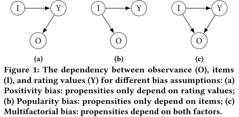
fixed user u에 대하여, item에 따라 preference score가 결정된다. \((I \rightarrow Y)\)
(Fig. 1a) Positivity bias에서는 preference score가 높을 수록 observation 확률 또한 높아진다. \((Y \rightarrow O)\)
따라서 rating score와 propensity가 비례해야 하므로, \[ Positivity-bias\left(\mathcal{D}\right) \Leftrightarrow Selection-bias\left(\mathcal{D}\right) \land \left(y_{u,i} > y_{u', i'} \leftrightarrow p_{u,i} > p_{u', i'}\right)\] 관계가 성립한다.
(Fig. 1b) 한편, popularity bias의 경우, user와 무관하게 item이 인기있을 수록 observation 확률이 커진다. \((I \rightarrow O)\)
따라서 동일한 item에 대하여 propensity score가 같아야 하므로,
\[ Popularity-bias\left(\mathcal{D}\right) \Leftrightarrow Selection-bias\left(\mathcal{D}\right) \land \left( i=i' \rightarrow p_{u,i} = p_{u', i'}\right)\] 관계가 성립한다.
2.2.4 Multi-factorial Bias
(Fig. 1c) 결과적으로, 본 논문에서는 주요 bias를 모두 고려한, Multi-factorial Bias 모형을 사용한다.
따라서 \((Y \rightarrow O), (I \rightarrow O)\)를 모두 고려해야 한다. \[ Multifactorial-bias\left(\mathcal{D}\right) \Leftrightarrow Selection-bias\left(\mathcal{D}\right) \land \left( i=i' \land y_{u,i} = y_{u', i'}\rightarrow p_{u,i} = p_{u', i'}\right)\]
2.3 Loss functions & Estimation
- Loss function의 경우 observations들을 통해 계산함을 유념하면, preference \(y\)가 아닌 rating \(r\)로 계산됨을 이해할 수 있다.
2.3.1 Naive Loss
Actual preference score인 \(y_{u,i}\)와 Predicted preference score인 \(\hat{y}_{u,i}\)간의 오차를 이용하여 loss function을 만들 수 있다.
MSE와 같은 오차 함수 \(\delta(\hat{y}_{u,i}, y_{u,i})\)를 사용하여, (사실 통계적으로는 잔차 함수이다. prediction - observation 이라서.) \[\mathcal{L} = \frac{1}{|\mathcal{U}||\mathcal{I}|}\sum_{u \in \mathcal{U}} \sum_{i \in \mathcal{I}} \delta(\hat{y}_{u,i}, y_{u,i}) \] 와 같은 방식이다.
그러나, 모든 (user, item) pair에서 actual preference score을 구할 수 없기 때문에, ideal loss인 \(\mathcal{L}\)을 구할 수 없다.
따라서 우리는 logged rating dataset인 \(\mathcal{D}\)에서 rating score인 \(r_{u,i}\)를 활용하여, loss function을 계산한다.
\[\mathcal{L}_{\text{Naive}}
= \frac{1}{|\mathcal{D}|}\sum_{u,i \in \mathcal{D}} \delta(\hat{y}_{u,i}, y_{u,i})
=\frac{1}{|\mathcal{D}|}\sum_{u,i \in \mathcal{D}} \delta(\hat{r}_{u,i}, r_{u,i})
\]
한편, rating dataset인 \(\mathcal{D}\)마다 \(\mathcal{L}_{\text{Naive}}\) 값이 달라지기 때문에,
우리는 이것의 기댓값인 \(\mathbb{E}\mathcal{L}_{\text{Naive}} = \frac{1}{|\mathcal{D}|}\sum_{u \in \mathcal{U}} \sum_{i \in \mathcal{I}} p_{u,i} \cdot \delta(\hat{y}_{u,i}, y_{u,i})\) 를 사용할 수 있다.
그러나 이러한 naive loss function은 앞에서 논의한 selection bias를 전혀 반영하지 못하기 때문에, IPS loss를 사용한다.
2.3.2 IPS(Inverse Propensity Scoring) Loss
IPS method는 selection bias 효과를 줄이기 위해 자주 사용된다. propensity score가 높은 (user, item) pair는 그만큼 rating 확률이 크기 때문에, 오차 함수의 값을 줄여주는 가중치를 적용해야 한다.
따라서 이러한 가중치를 propensity socre의 역수를 적용함으로서, \(\mathcal{L}_{\text{IPS}} = \frac{1}{|\mathcal{U}||\mathcal{I}|}\sum_{u,i \in \mathcal{D}}\frac{1}{p_{u,i}}\delta(\hat{r}_{u,i}, r_{u,i})\) 로 IPS loss를 정의한다.
이 때, 위와 같은 논리로 기댓값을 적용하여 이러한 IPS loss의 평균을 내면, \[ \begin{aligned} \mathbb{E}\mathcal{L}_{\text{IPS}} &= \mathbb{E}\frac{1}{|\mathcal{U}||\mathcal{I}|}\sum_{u,i \in \mathcal{D}} \frac{1}{p_{u,i}}\delta(\hat{r}_{u,i}, r_{u,i}) \\ &= \mathbb{E}\frac{1}{|\mathcal{U}||\mathcal{I}|}\sum_{u \in \mathcal{U}} \sum_{i \in \mathcal{I}} o_{u,i}\frac{1}{p_{u,i}}\delta(\hat{y}_{u,i}, y_{u,i}) \\ &= \frac{1}{|\mathcal{U}||\mathcal{I}|}\sum_{u \in \mathcal{U}} \sum_{i \in \mathcal{I}}\frac{\mathbb{E} o_{u,i}}{p_{u,i}}\delta(\hat{y}_{u,i}, y_{u,i}) \\ &= \frac{1}{|\mathcal{U}||\mathcal{I}|}\sum_{u \in \mathcal{U}} \sum_{i \in \mathcal{I}}\delta(\hat{y}_{u,i}, y_{u,i}) \quad \left(\because \mathbb{E} o_{u,i}=1*p_{u,i} + 0*(1-p_{u,i}) = p_{u,i} \right) \\ &= \mathcal{L} \end{aligned} \]
와 같이 정리된다.
=> 따라서 임의의 \(\mathcal{D}\)에 대하여 \(\mathcal{L}_{\text{IPS}}\)를 계산할 수 있다면, 평균을 통해 ideal loss인 \(\mathcal{L}\)을 구할 수 있다.
2.3.3 Propensity Estimation
한편, \(\mathcal{L}_{\text{IPS}}\)를 구하기 위해 propensity score \(p_{u,i}\)를 알아내야 하지만, 모집단의 분포를 모르기 때문에 이 또한 추정해야만 한다.
참고로, PROPCARE에서는 popularity에만 의존하는 single-factor bias 관점에서 propensity를 추정하였다.
기존의 다른 연구 또한 positivity or popularity bias에만 의존한다는 관점에서 propensity를 추정하였으나, 본 논문에서는 둘 모두를 고려하는 Milti-factorial bias관점을 채택한다.
- positivity bias 관점에서, \(\hat{p}_{u,i}^{\text{pos}}=P\left(o=1 | y=y_{u,i}\right)\)
- popularity bias 관점에서, \(\hat{p}_{u,i}^{\text{pop}}=P\left(o=1 | i \right)\) \(\leftarrow\) item = i 일 때
따라서 최종적으로 multi-factorial bias 관점에서 propensity score를 추정하면, 아래와 같다.
\[
\hat{p}_{u,i}^{\text{mul}}=P\left(o=1 | y=y_{u,i}, i \right)=\frac{P\left(y=y_{u,i}, i | o=1 \right)P\left(o=1\right)}{P\left(y=y_{u,i}, i \right)}
\]
이 때 data sparsity 문제를 해결하기 위해 Laplace smoothing 등 근사를 통하여 \(\hat{p}_{u,i}^{\text{mul}}\)를 구한다.
2.3.4 Predicted rating score \(\hat{y}_{u,i} Estimation\)
\(\hat{y}_{u,i}\)의 경우 본 논문에서는 standard Matrix Factorization (MF) model을 사용한다. \[ \hat{y}_{u,i} = p_u ^T q_i + a_u + b_i + c, \quad \Theta = \{p_u, q_i, a_u, b_i, c\} \] 다른 방법을 사용해도 무방하다.
2.3.5 Total Loss function
이제, 마지막으로 Total Loss function을 구해야 한다.
\(\mathcal{L}_{\text{IPS}}\)의 기댓값이 ideal loss \(\mathcal{L}\)로 좋은 결과를 가져오기 때문에, \(\mathcal{L}_{\text{IPS}}\)를 원형으로 total loss를 구한다.
먼저, \(p, y\)에 대해 추정값을 사용한 IPS loss를 구하면, (\(\hat{y}\)의 경우 MF를 사용.) \[ \mathcal{L}_{\text{MF-IPS}^{\text{Mul}}} = \frac{1}{|\mathcal{D}|}\sum_{u,i \in \mathcal{D}} \frac{1}{\hat{p}_{u,i}^{\text{mul}}}\delta(\hat{y}_{u,i}, y_{u,i}) \] 이다.
이 때 overfitting을 막기 위해 \(L_2\)-regularization term을 넣으면, Total Loss는 아래와 같다. \[ \begin{aligned} \mathcal{L}_{\text{total}} &= \mathcal{L}_{\text{MF-IPS}^{\text{Mul}}} \left(\Theta\right) \\ &= \frac{1}{|\mathcal{D}|}\sum_{u,i \in \mathcal{D}} \frac{1}{\hat{p}_{u,i}^{\text{mul}}}\delta(\hat{y}_{u,i}, y_{u,i}) + \lambda||\Theta||_2 ^2\\ \end{aligned} \]
- 논문에서는 예시로 \(\delta(\hat{y}_{u,i}, y_{u,i})=(\hat{y}_{u,i} - y_{u,i})^2\) 와 같은 MSE로 설명하였지만, 이후 Table 1에서 볼 수 있듯이 다른 오차 함수를 사용할 수 있다.
3 Method (Solution)
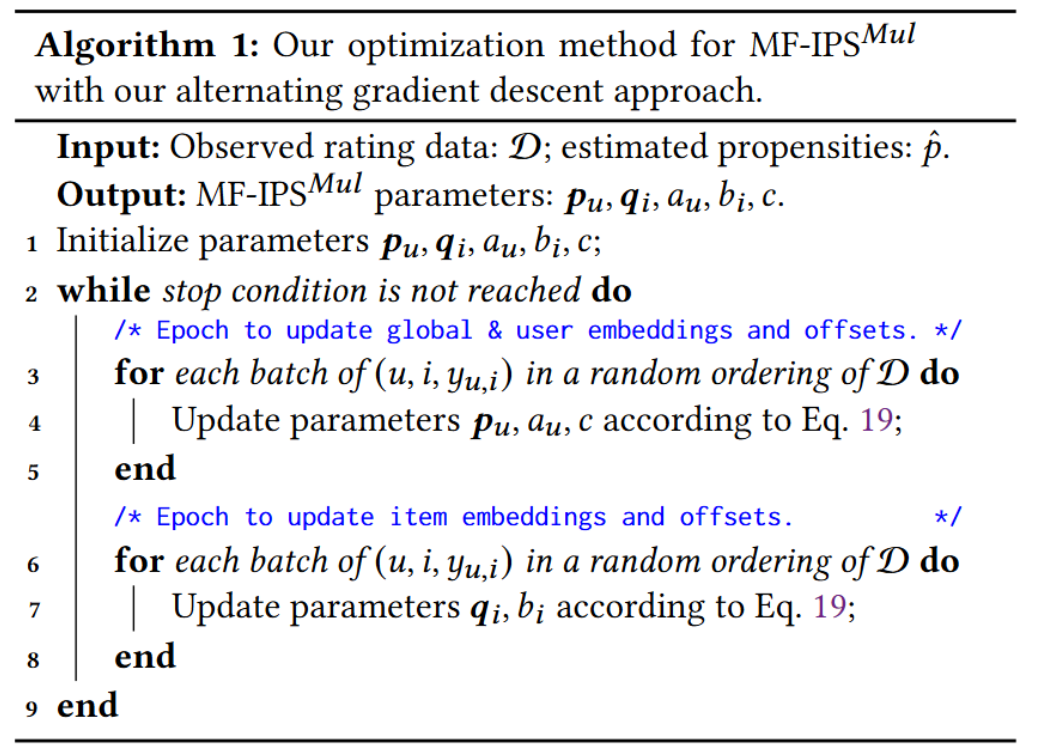
- For updating our parameters \(\theta \in \Theta\), we use alternating gradient descent algorithm and Adam optimizer.
- Eq. 19: \(\quad \theta_{t} = \text{ADAM}\left(\theta_{t-1}, \nabla\theta_{t-1} \mathcal{L}_{\text{MF-IPS}^{\text{Mul}}}\right)\)
4 Experiments & Result
RQ1: Does our proposed multifactorial method better mitigate the effect of bias in logged rating data than existing single-factor debiasing methods?
(RQ2) How do varying smoothing parameters and our alternating gradient descent approach affect our multifactorial method?
(RQ3) Can our multifactorial method \(\text{MF-IPS}^{\text{Mul}}\) robustly mitigate the effect of selection bias in scenarios where the effect of two factors on bias is varied?
4.1 Datasets
4.2 Error Function \(\delta(\hat{y}_{u,i}, y_{u,i})\)
- mean squared error (MSE)
- mean absolute error (MAE)
- root mean square error (RMSE)
- average RMSE performance per user (\(\text{RMSE}_𝑈\))
- average RMSE performance per item (\(\text{RMSE}_I\))
- RMSE score for each individual user/item separately and then average them.
4.3 Baselines (Methods) in Single-factor bias
- No IPS model, Ignore any selection bias
- Avg model
- MF model
- VAE model
- IPS model, De-biased method
- \(\text{MF-IPS}^{\text{MF}}\): MF model - propensity estimation using MF with logistic regression
- \(\text{MF-IPS}^{\text{Pop}}\): MF model with \(\hat{p}_{u,i}^{\text{pop}}\)
- \(\text{MF-IPS}^{\text{Pos}}\): MF model with \(\hat{p}_{u,i}^{\text{pos}}\)
Paper: Multi-factorial Bias \(\text{MF-IPS}^{\text{Mul}}\): MF model with \(\hat{p}_{u,i}^{\text{mul}}\)
4.4 Hyper-parameters tuning
4.4.1 In the MF-based methods
- learning rate: \(\eta\)
- \(L_2\) regularization weights: \(\lambda\)
- dimension of embeddings of users and items: \(d\)
4.4.2 In the VAE method
- learning rate
- regularization weights
- dimension of the latent representation
- Kullback-Leibler term
4.4.3 Paper method (multi-factorial bias)
- learning rate: \(\eta\)
- \(L_2\) regularization weights: \(\lambda\)
- dimension of embeddings of users and items: \(d\)
- smoothing parameters: \(\alpha_1, \alpha_2\)
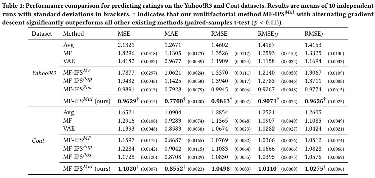
4.5 RQ1 Answer: [Model Performance]
RQ1: Does our proposed multifactorial method better mitigate the effect of bias in logged rating data than existing single-factor debiasing methods?
- Yes. 모든 Error Function \(\delta\)에서 paper의 모형이 가장 Error evaluation이 낮다. 두 dataset 모두
- \(\text{MF-IPS}^{\text{Mul}} \succ \text{MF-IPS}^{\text{Pos}} \succ \text{MF-IPS}^{\text{Pop}}\): positivity bias has a stronger effect than popularity bias in rating predictions.
4.6 RQ2 Answer: [Alternating GD & Smoothing]
(RQ2) How do varying smoothing parameters and our alternating gradient descent approach affect our multifactorial method?
- 나중에 작성. (논문 5.3)
4.7 RQ3 Answer: [Robustness]
(RQ3) Can our multifactorial method \(\text{MF-IPS}^{\text{Mul}}\) robustly mitigate the effect of selection bias in scenarios where the effect of two factors on bias is varied?
- 나중에 작성. (논문 6.1-6.2)
5 Conclusion
Multi-factorial Selection Bias \(\text{MF-IPS}^{\text{Mul}}\): MF model with \(\hat{p}_{u,i}^{\text{mul}}\) \(\leftarrow\) Popularity bias & Positivity bias
- Better Performance
- More Stable from the data sparsity problem
- More Robust
than SOTA (Single-factor Selection Bias model)